Em matemática , uma série de Taylor é a série de funções da forma:
f
(
x
)
=
∑
n
=
0
∞
a
n
(
x
−
a
)
n
sendo
a
n
=
f
(
n
)
(
a
)
n
!
{\displaystyle f(x)=\sum _{n=0}^{\infty }a_{n}(x-a)^{n}\quad {\mbox{sendo}}\quad a_{n}={\frac {f^{(n)}(a)}{n!}}}
onde
f
(
x
)
{\textstyle f(x)}
f
(
x
)
{\textstyle f(x)}
x
=
a
{\textstyle x=a}
polinômio de Taylor de ordem
n
{\textstyle n}
em torno de
x
=
a
{\textstyle x=a}
n
{\textstyle n}
[ 1] [ 2] [ 3] [ 4] [ 5] [ 6] [ 7] [ 8]
p
(
x
)
=
f
(
a
)
+
f
′
(
a
)
(
x
−
a
)
1
1
!
+
f
″
(
a
)
(
x
−
a
)
2
2
!
+
.
.
.
+
f
(
n
)
(
a
)
(
x
−
a
)
n
n
!
{\displaystyle p(x)=f(a)+f'(a){\frac {\left(x-a\right)^{1}}{1!}}+f''(a){\frac {\left(x-a\right)^{2}}{2!}}+...+f^{(n)}(a){\frac {\left(x-a\right)^{n}}{n!}}}
No caso particular de
a
=
0
{\textstyle a=0}
, série acima também é chamada de Série de Maclaurin
Tais séries recebem seu nome em homenagem a Brook Taylor que as estudou no trabalho Methodus incrementorum directa et inversa em 1715 . Condorcet atribuía estas séries a Taylor e d'Alembert . O nome série de Taylor só começou a ser usado em 1786, por l'Huillier.
Toda série de Taylor possui um raio de convergência
R
{\displaystyle R}
circunferência )
|
x
−
a
|
≤
r
<
R
{\displaystyle |x-a|\leq r<R}
A fórmula de Hadamard fornece o valor deste raio de convergência:
R
−
1
=
lim sup
n
→
∞
|
a
n
|
1
/
n
{\displaystyle R^{-1}=\limsup _{n\to \infty }|a_{n}|^{1/n}}
O fato de a série de Taylor convergir não garante que ela convergirá para o valor da função f(x); o exemplo clássico desta patologia é a função definida por:
f
(
x
)
=
{
exp
(
−
1
/
x
)
se
x
>
0
,
0
se
x
≤
0
,
{\displaystyle f(x)={\begin{cases}\exp(-1/x)&{\text{se }}x>0,\\0&{\text{se }}x\leq 0,\end{cases}}}
cuja série de Taylor é :
f
(
x
)
=
0
+
0
x
+
0
x
2
+
…
{\displaystyle f(x)=0+0x+0x^{2}+\ldots }
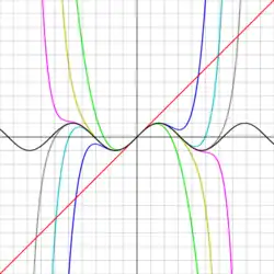
Função seno de x e aproximações de Taylor com polinômios de grau 1 , 3 , 5 , 7 , 9 , 11 e 13 .[ 9] A série de Taylor associada a uma função
f
{\displaystyle f}
infinitamente diferenciável (real ou complexa ) definida em um intervalo aberto ]a − r , a + r [ é a série de potências dada por
f
(
x
)
=
∑
n
=
0
∞
f
(
n
)
(
a
)
n
!
(
x
−
a
)
n
.
{\displaystyle f(x)=\sum _{n=0}^{\infty }{\frac {f^{(n)}(a)}{n!}}(x-a)^{n}.}
Onde, n ! é o fatorial de n e f (n ) (a ) denota a n -ésima derivada de f no ponto a .
Com essa ferramenta, podem ser moldadas funções trigonométricas, exponenciais e logarítmicas em polinômios .
a
=
0
{\textstyle a=0}
Função exponencial e logaritmo natural :
e
x
=
∑
n
=
0
∞
x
n
n
!
para todo
x
{\displaystyle \mathrm {e} ^{x}=\sum _{n=0}^{\infty }{\frac {x^{n}}{n!}}\quad {\mbox{ para todo }}x}
[ 10]
ln
(
1
+
x
)
=
∑
n
=
0
∞
(
−
1
)
n
n
+
1
x
n
+
1
para
|
x
|
<
1
{\displaystyle \ln(1+x)=\sum _{n=0}^{\infty }{\frac {(-1)^{n}}{n+1}}x^{n+1}\quad {\mbox{ para }}\left|x\right|<1}
Série geométrica :
x
m
1
−
x
=
∑
n
=
m
∞
x
n
para
|
x
|
<
1
{\displaystyle {\frac {x^{m}}{1-x}}=\sum _{n=m}^{\infty }x^{n}\quad {\mbox{ para }}\left|x\right|<1}
Teorema binomial :
(
1
+
x
)
α
=
∑
n
=
0
α
(
α
n
)
x
n
para todo
|
x
|
<
1
e todo complexo
α
{\displaystyle (1+x)^{\alpha }=\sum _{n=0}^{\alpha }{\alpha \choose n}x^{n}\quad {\mbox{ para todo }}\left|x\right|<1\quad {\mbox{ e todo complexo }}\alpha }
Funções trigonométricas :
cos
x
=
∑
n
=
0
∞
(
−
1
)
n
(
2
n
)
!
x
2
n
para todo
x
{\displaystyle \cos x=\sum _{n=0}^{\infty }{\frac {(-1)^{n}}{(2n)!}}x^{2n}\quad {\mbox{ para todo }}x}
sin
x
=
∑
n
=
0
∞
(
−
1
)
n
(
2
n
+
1
)
!
x
2
n
+
1
para todo
x
{\displaystyle \sin x=\sum _{n=0}^{\infty }{\frac {(-1)^{n}}{(2n+1)!}}x^{2n+1}\quad {\mbox{ para todo }}x}
tan
x
=
∑
n
=
1
∞
B
2
n
(
−
4
)
n
(
1
−
4
n
)
(
2
n
)
!
x
2
n
−
1
=
x
+
x
3
3
+
2
x
5
15
+
.
.
para
|
x
|
<
π
2
{\displaystyle \tan x=\sum _{n=1}^{\infty }{\frac {B_{2n}(-4)^{n}(1-4^{n})}{(2n)!}}x^{2n-1}\quad =x+{\frac {x^{3}}{3}}+{\frac {2x^{5}}{15}}+..{\mbox{ para }}\left|x\right|<{\frac {\pi }{2}}}
onde B k
sec
x
=
∑
n
=
0
∞
(
−
1
)
n
E
2
n
(
2
n
)
!
x
2
n
para
|
x
|
<
π
2
{\displaystyle \sec x=\sum _{n=0}^{\infty }{\frac {(-1)^{n}E_{2n}}{(2n)!}}x^{2n}\quad {\mbox{ para }}\left|x\right|<{\frac {\pi }{2}}}
onde E k
arcsin
x
=
∑
n
=
0
∞
(
2
n
)
!
4
n
(
n
!
)
2
(
2
n
+
1
)
x
2
n
+
1
para
|
x
|
<
1
{\displaystyle \arcsin x=\sum _{n=0}^{\infty }{\frac {(2n)!}{4^{n}(n!)^{2}(2n+1)}}x^{2n+1}\quad {\mbox{ para }}\left|x\right|<1}
arctan
x
=
∑
n
=
0
∞
(
−
1
)
n
2
n
+
1
x
2
n
+
1
para
|
x
|
<
1
{\displaystyle \arctan x=\sum _{n=0}^{\infty }{\frac {(-1)^{n}}{2n+1}}x^{2n+1}\quad {\mbox{ para }}\left|x\right|<1}
Funções hiperbólicas :
sinh
(
x
)
=
∑
n
=
0
∞
1
(
2
n
+
1
)
!
x
2
n
+
1
para todo
x
{\displaystyle \sinh \left(x\right)=\sum _{n=0}^{\infty }{\frac {1}{(2n+1)!}}x^{2n+1}\quad {\mbox{ para todo }}x}
cosh
(
x
)
=
∑
n
=
0
∞
1
(
2
n
)
!
x
2
n
para todo
x
{\displaystyle \cosh \left(x\right)=\sum _{n=0}^{\infty }{\frac {1}{(2n)!}}x^{2n}\quad {\mbox{ para todo }}x}
tanh
(
x
)
=
∑
n
=
1
∞
B
2
n
4
n
(
4
n
−
1
)
(
2
n
)
!
x
2
n
−
1
para
|
x
|
<
π
2
{\displaystyle \tanh \left(x\right)=\sum _{n=1}^{\infty }{\frac {B_{2n}4^{n}(4^{n}-1)}{(2n)!}}x^{2n-1}\quad {\mbox{ para }}\left|x\right|<{\frac {\pi }{2}}}
a
r
c
s
e
n
h
(
x
)
=
∑
n
=
0
∞
(
−
1
)
n
(
2
n
)
!
4
n
(
n
!
)
2
(
2
n
+
1
)
x
2
n
+
1
para
|
x
|
<
1
{\displaystyle \mathrm {arcsenh} \left(x\right)=\sum _{n=0}^{\infty }{\frac {(-1)^{n}(2n)!}{4^{n}(n!)^{2}(2n+1)}}x^{2n+1}\quad {\mbox{ para }}\left|x\right|<1}
a
r
c
t
a
n
h
(
x
)
=
∑
n
=
0
∞
1
2
n
+
1
x
2
n
+
1
para
|
x
|
<
1
{\displaystyle \mathrm {arctanh} \left(x\right)=\sum _{n=0}^{\infty }{\frac {1}{2n+1}}x^{2n+1}\quad {\mbox{ para }}\left|x\right|<1}
Função W de Lambert:
W
0
(
x
)
=
∑
n
=
1
∞
(
−
n
)
n
−
1
n
!
x
n
para
|
x
|
<
1
e
{\displaystyle W_{0}(x)=\sum _{n=1}^{\infty }{\frac {(-n)^{n-1}}{n!}}x^{n}\quad {\mbox{ para }}\left|x\right|<{\frac {1}{\mathrm {e} }}}
A série de Taylor pode também ser definida para funções de
R
n
→
R
{\displaystyle \mathbb {R} ^{n}\rightarrow \mathbb {R} }
Nesse caso, tem-se que a série de Taylor de
f
{\displaystyle f}
X
0
=
(
x
1
0
,
⋯
,
x
n
0
)
{\displaystyle X_{0}=(x_{1}^{0},\cdots ,x_{n}^{0})}
f
(
x
1
,
⋯
,
x
n
)
=
∑
k
≥
0
1
k
!
(
∑
i
=
1
n
∂
f
∂
x
i
(
X
0
)
(
x
i
−
x
i
0
)
)
k
,
{\displaystyle f(x_{1},\cdots ,x_{n})=\sum \limits _{k\geq 0}{\frac {1}{k!}}\left(\sum \limits _{i=1}^{n}{\frac {\partial f}{\partial x_{i}}}(X_{0})(x_{i}-x_{i}^{0})\right)^{k},}
onde
(
∂
f
∂
x
i
(
X
0
)
)
k
{\displaystyle \left({\frac {\partial f}{\partial x_{i}}}(X_{0})\right)^{k}}
∂
k
f
∂
x
i
k
(
X
0
)
.
{\displaystyle {\frac {\partial ^{k}f}{\partial x_{i}^{k}}}(X_{0}).}
Ou seja, tem-se:
(
∑
i
=
1
n
∂
f
∂
x
i
(
X
0
)
(
x
i
−
x
i
0
)
)
k
=
∑
α
i
∈
N
,
∑
i
=
1
n
α
i
=
k
(
k
!
α
1
!
⋯
α
n
!
⋅
∂
k
f
∂
x
1
α
1
⋯
∂
x
n
α
n
(
X
0
)
⋅
(
x
1
−
x
1
0
)
α
1
⋯
(
x
n
−
x
n
0
)
α
n
)
.
{\displaystyle \left(\sum \limits _{i=1}^{n}{\frac {\partial f}{\partial x_{i}}}(X_{0})(x_{i}-x_{i}^{0})\right)^{k}=\sum \limits _{\alpha _{i}\in \mathbb {N} ,\sum \limits _{i=1}^{n}\alpha _{i}=k}\left({\frac {k!}{\alpha _{1}!\cdots \alpha _{n}!}}\cdot {\frac {\partial ^{k}f}{\partial x_{1}^{\alpha _{1}}\cdots \partial x_{n}^{\alpha _{n}}}}(X_{0})\cdot (x_{1}-x_{1}^{0})^{\alpha _{1}}\cdots (x_{n}-x_{n}^{0})^{\alpha _{n}}\right).}
No caso particular
n
=
2
{\displaystyle n=2}
X
0
=
(
x
0
,
y
0
)
:
{\displaystyle X_{0}=(x_{0},y_{0}):}
f
(
x
,
y
)
=
∑
k
≥
0
1
k
!
∑
i
=
0
k
k
!
i
!
(
k
−
i
)
!
⋅
∂
i
f
∂
x
i
(
X
0
)
⋅
∂
k
−
i
f
∂
y
k
−
i
(
X
0
)
⋅
(
x
−
x
0
)
i
⋅
(
y
−
y
0
)
k
−
i
.
{\displaystyle f(x,y)=\sum \limits _{k\geq 0}{\frac {1}{k!}}\sum \limits _{i=0}^{k}{\frac {k!}{i!(k-i)!}}\cdot {\frac {\partial ^{i}f}{\partial x^{i}}}(X_{0})\cdot {\frac {\partial ^{k-i}f}{\partial y^{k-i}}}(X_{0})\cdot (x-x_{0})^{i}\cdot (y-y_{0})^{k-i}.}
[ 11]
As Séries de Maclaurin são um caso especial das Séries de Taylor onde
a
=
0
{\displaystyle a=0}
f
(
x
)
=
∑
n
=
0
∞
f
(
n
)
(
a
)
(
x
−
a
)
n
n
!
{\displaystyle f(x)=\sum _{n=0}^{\infty }{f^{(n)}(a)(x-a)^{n} \over n!}}
Dessa forma, a série pode ser expandida como:
f
(
x
)
=
f
(
0
)
(
x
−
0
)
0
+
f
′
(
0
)
(
x
−
0
)
1
1
!
+
f
″
(
0
)
(
x
−
0
)
2
2
!
+
f
‴
(
0
)
(
x
−
0
)
3
3
!
+
.
.
.
{\displaystyle f(x)=f(0)(x-0)^{0}+{f'(0)(x-0)^{1} \over 1!}+{f''(0)(x-0)^{2} \over 2!}+{f'''(0)(x-0)^{3} \over 3!}+...}
Logo:
f
(
x
)
=
f
(
0
)
+
f
′
(
0
)
x
1
1
!
+
f
″
(
0
)
x
2
2
!
+
f
‴
(
0
)
x
3
3
!
+
.
.
.
{\displaystyle f(x)=f(0)+{f'(0)\ x^{1} \over 1!}+{f''(0)\ x^{2} \over 2!}+{f'''(0)\ x^{3} \over 3!}+...}
Escrevendo-se a Série da Maclaurin de forma geral:
f
(
x
)
=
∑
n
=
0
∞
f
(
n
)
(
0
)
x
n
n
!
{\displaystyle f(x)=\sum _{n=0}^{\infty }{f^{(n)}(0)\ x^{n} \over n!}}
s
e
n
(
x
)
{\displaystyle sen(x)}
Para o
c
o
s
(
x
)
{\displaystyle cos(x)}
f
(
x
)
=
s
e
n
(
x
)
⇒
f
(
0
)
=
s
e
n
(
0
)
=
0
{\displaystyle f(x)=sen(x)\Rightarrow f(0)=sen(0)=0}
Derivadas
f
′
(
x
)
=
c
o
s
(
x
)
⇒
f
′
(
0
)
=
c
o
s
(
0
)
=
1
{\displaystyle f'(x)=cos(x)\Rightarrow f'(0)=cos(0)=1}
f
″
(
x
)
=
−
s
e
n
(
x
)
⇒
f
″
(
0
)
=
−
s
e
n
(
0
)
=
−
0
=
0
{\displaystyle f''(x)=-sen(x)\Rightarrow f''(0)=-sen(0)=-0=0}
f
‴
(
x
)
=
−
c
o
s
(
x
)
⇒
f
‴
(
0
)
=
−
c
o
s
(
0
)
=
−
1
{\displaystyle f'''(x)=-cos(x)\Rightarrow f'''(0)=-cos(0)=-1}
f
⁗
(
x
)
=
s
e
n
(
x
)
⇒
f
⁗
(
0
)
=
s
e
n
(
0
)
=
0
{\displaystyle f''''(x)=sen(x)\Rightarrow f''''(0)=sen(0)=0}
f
′′′′′
(
x
)
=
c
o
s
(
x
)
⇒
f
′′′′′
(
0
)
=
c
o
s
(
0
)
=
1
{\displaystyle f'''''(x)=cos(x)\Rightarrow f'''''(0)=cos(0)=1}
f
′′′′′′
(
x
)
=
−
s
e
n
(
x
)
⇒
f
′′′′′′
(
0
)
=
−
s
e
n
(
0
)
=
−
0
=
0
{\displaystyle f''''''(x)=-sen(x)\Rightarrow f''''''(0)=-sen(0)=-0=0}
f
′′′′′′′
(
x
)
=
−
c
o
s
(
x
)
⇒
f
′′′′′′′
(
0
)
=
−
c
o
s
(
0
)
=
−
1
{\displaystyle f'''''''(x)=-cos(x)\Rightarrow f'''''''(0)=-cos(0)=-1}
f
′′′′′′′′
(
x
)
=
s
e
n
(
x
)
⇒
f
′′′′′′′′
(
0
)
=
s
e
n
(
0
)
=
0
{\displaystyle f''''''''(x)=sen(x)\Rightarrow f''''''''(0)=sen(0)=0}
f
′′′′′′′′′
(
x
)
=
c
o
s
(
x
)
⇒
f
′′′′′′′′′
(
0
)
=
c
o
s
(
0
)
=
1
{\displaystyle f'''''''''(x)=cos(x)\Rightarrow f'''''''''(0)=cos(0)=1}
Substituindo-se as derivadas na série, tem-se que:
f
(
x
)
=
f
(
0
)
+
f
′
(
0
)
x
1
1
!
+
f
″
(
0
)
x
2
2
!
+
f
‴
(
0
)
x
3
3
!
+
f
⁗
(
0
)
x
4
4
!
+
f
′′′′′
(
0
)
x
5
5
!
+
f
′′′′′′
(
0
)
x
6
6
!
+
f
′′′′′′′
(
0
)
x
7
7
!
+
f
′′′′′′′′
(
0
)
x
8
8
!
+
f
′′′′′′′′′
(
0
)
x
9
9
!
{\displaystyle f(x)=f(0)+{f'(0)\ x^{1} \over 1!}+{f''(0)\ x^{2} \over 2!}+{f'''(0)\ x^{3} \over 3!}+{f''''(0)\ x^{4} \over 4!}+{f'''''(0)\ x^{5} \over 5!}+{f''''''(0)\ x^{6} \over 6!}+{f'''''''(0)\ x^{7} \over 7!}+{f''''''''(0)\ x^{8} \over 8!}+{f'''''''''(0)\ x^{9} \over 9!}}
Observa-se, que as derivadas segunda, quarta, sexta e oitava. Logo, os termos da série com
x
{\displaystyle x}
f
(
x
)
≅
(
1
x
1
1
!
)
+
(
−
1
x
3
3
!
)
+
(
1
x
5
5
!
)
+
(
−
1
x
7
7
!
)
+
(
1
x
9
9
!
)
{\displaystyle f(x)\cong \left({1x^{1} \over 1!}\right)+\left({-1x^{3} \over 3!}\right)+\left({1x^{5} \over 5!}\right)+\left({-1x^{7} \over 7!}\right)+\left({1x^{9} \over 9!}\right)}
Realizando-se a multiplicação e simplificando os expoentes:
f
(
x
)
≅
x
−
x
3
3
!
+
x
5
5
!
−
x
7
7
!
+
x
9
9
!
{\displaystyle f(x)\cong x\ -{x^{3} \over 3!}+\ {x^{5} \over 5!}\ -{x^{7} \over 7!}+\ {x^{9} \over 9!}}
Dessa forma, a série pode ser escrita como:
f
(
x
)
=
s
e
n
(
x
)
=
∑
n
=
0
∞
(
−
1
)
n
x
2
n
+
1
(
2
n
+
1
)
!
{\displaystyle f(x)=sen(x)=\sum _{n=0}^{\infty }(-1)^{n}{x^{2n+1} \over (2n+1)!}}
c
o
s
(
x
)
{\displaystyle cos(x)}
Para o
c
o
s
(
x
)
{\displaystyle cos(x)}
f
(
x
)
=
c
o
s
(
x
)
⇒
f
(
0
)
=
c
o
s
(
0
)
=
1
{\displaystyle f(x)=cos(x)\Rightarrow f(0)=cos(0)=1}
Derivadas
f
′
(
x
)
=
−
s
e
n
(
x
)
⇒
f
′
(
0
)
=
−
s
e
n
(
0
)
=
−
0
=
0
{\displaystyle f'(x)=-sen(x)\Rightarrow f'(0)=-sen(0)=-0=0}
f
″
(
x
)
=
−
c
o
s
(
x
)
⇒
f
″
(
0
)
=
−
c
o
s
(
0
)
=
−
1
{\displaystyle f''(x)=-cos(x)\Rightarrow f''(0)=-cos(0)=-1}
f
‴
(
x
)
=
s
e
n
(
x
)
⇒
f
‴
(
0
)
=
s
e
n
(
0
)
=
0
{\displaystyle f'''(x)=sen(x)\Rightarrow f'''(0)=sen(0)=0}
f
⁗
(
x
)
=
c
o
s
(
x
)
⇒
f
⁗
(
0
)
=
c
o
s
(
0
)
=
1
{\displaystyle f''''(x)=cos(x)\Rightarrow f''''(0)=cos(0)=1}
f
′′′′′
(
x
)
=
−
s
e
n
(
x
)
⇒
f
′′′′′
(
0
)
=
−
s
e
n
(
0
)
=
−
0
=
0
{\displaystyle f'''''(x)=-sen(x)\Rightarrow f'''''(0)=-sen(0)=-0=0}
f
′′′′′′
(
x
)
=
−
c
o
s
(
x
)
⇒
f
′′′′′′
(
0
)
=
−
c
o
s
(
0
)
=
−
1
{\displaystyle f''''''(x)=-cos(x)\Rightarrow f''''''(0)=-cos(0)=-1}
f
′′′′′′′
(
x
)
=
s
e
n
(
x
)
⇒
f
′′′′′′′
(
0
)
=
s
e
n
(
0
)
=
0
{\displaystyle f'''''''(x)=sen(x)\Rightarrow f'''''''(0)=sen(0)=0}
f
′′′′′′′′
(
x
)
=
c
o
s
(
x
)
⇒
f
′′′′′′′′
(
0
)
=
c
o
s
(
0
)
=
1
{\displaystyle f''''''''(x)=cos(x)\Rightarrow f''''''''(0)=cos(0)=1}
f
′′′′′′′′′
(
x
)
=
−
s
e
n
(
x
)
⇒
f
′′′′′′′′′
(
0
)
=
−
s
e
n
(
0
)
=
−
0
=
0
{\displaystyle f'''''''''(x)=-sen(x)\Rightarrow f'''''''''(0)=-sen(0)=-0=0}
f
′′′′′′′′′′
(
x
)
=
−
c
o
s
(
x
)
⇒
f
′′′′′′′′′′
(
0
)
=
−
c
o
s
(
0
)
=
−
1
{\displaystyle f''''''''''(x)=-cos(x)\Rightarrow f''''''''''(0)=-cos(0)=-1}
f
′′′′′′′′′′′
(
x
)
=
s
e
n
(
x
)
⇒
f
′′′′′′′′′′′
(
0
)
=
s
e
n
(
0
)
=
0
{\displaystyle f'''''''''''(x)=sen(x)\Rightarrow f'''''''''''(0)=sen(0)=0}
Observa-se, que as derivadas primeira, terceira, quinta, sétima e nona são iguais à zero. Logo, os termos da série com
x
{\displaystyle x}
f
(
x
)
≅
f
(
0
)
x
0
0
!
+
f
″
(
0
)
x
2
2
!
+
f
⁗
(
0
)
x
4
4
!
+
f
′′′′′′
(
0
)
x
6
6
!
+
f
′′′′′′′′
(
0
)
x
8
8
!
{\displaystyle f(x)\cong {f(0)x^{0} \over 0!}+{f''(0)x^{2} \over 2!}+{f''''(0)x^{4} \over 4!}+{f''''''(0)x^{6} \over 6!}+{f''''''''(0)x^{8} \over 8!}}
Substituindo-se os valores das derivadas e da
f
(
0
)
{\displaystyle f(0)}
f
(
x
)
≅
1
x
0
0
!
+
(
−
1
)
x
2
2
!
+
1
x
4
4
!
+
(
−
1
)
x
6
6
!
+
1
x
8
8
!
{\displaystyle f(x)\cong {1x^{0} \over 0!}+{(-1)x^{2} \over 2!}+{1x^{4} \over 4!}+{(-1)x^{6} \over 6!}+{1x^{8} \over 8!}}
Realizando-se a multiplicação e simplificando o 1° termo:
f
(
x
)
≅
1
−
x
2
2
!
+
x
4
4
!
−
x
6
6
!
+
x
8
8
!
{\displaystyle f(x)\cong 1-{x^{2} \over 2!}+{x^{4} \over 4!}-{x^{6} \over 6!}+{x^{8} \over 8!}}
Ou ainda:
f
(
x
)
=
cos
(
x
)
=
∑
n
=
0
∞
(
−
1
)
n
.
x
2
n
(
2
n
)
!
{\displaystyle f(x)=\cos(x)=\sum _{n=0}^{\infty }{(-1)^{n}.x^{2n} \over (2n)!}}
↑ Wolfram Alpha LLC—A Wolfram Research Company
↑ Sobre Desenvolvimentos em Séries de Potências, Séries de Taylor e Fórmula de Taylor ↑ Série de Taylor ↑ Notas de Aula MatLab Série, limite, equação diferencial ↑ Thomas, George B. Jr.; Finney, Ross L. (1996), Calculus and Analytic Geometry (9th ed.), Addison Wesley, ISBN 0-201-53174-7 (em inglês)
↑ Greenberg, Michael (1998), Advanced Engineering Mathematics (2nd ed.), Prentice Hall, ISBN 0-13-321431-1 (em inglês)
↑ Amos Gilat, Vish Subramaniam, Métodos Numéricos para Engenheiros e Cientistas: Uma Introdução com Aplicações Usando o MATLAB , Bookman, 2008 ISBN 8-577-80297-3
↑ Steven C. Chapra e Raymond P. Canale, Métodos Numéricos para Engenharia , McGraw Hill Brasil, 2011 ISBN 8-580-55011-4
↑ «Confira este exemplo e faça outros com O Monitor » . omonitor.io . Consultado em 23 de março de 2016 ↑ «Confira este exemplo e faça outros com O Monitor » . omonitor.io . Consultado em 23 de março de 2016 ↑ «Faça exemplos com O Monitor » . omonitor.io . Consultado em 23 de março de 2016
Alpha
Brook Taylor
Série de Laurent
Polinómio de Newton
Handbook of Mathematical Functions
Bibliografia
Heinrich Auchter. Brook Taylor, der mathematiker und philosoph; beiträge zur wissenschaftsgeschichte der zeit des Newton-Leibniz-streites, . Würzburg, K. Triltsch, 1937. OCLC 13481133
Edmundo Capelas de Oliveira, Funções Especiais com Aplicações , Editora Livraria da Fisica ISBN 8-588-32542-X
Steven C. Chapra, Métodos Numéricos Aplicados com MATLAB® para Engenheiros e Cientistas - 3.ed. McGraw Hill Brasil, 2013 ISBN 8-580-55177-3